
电脑excel点击单元格出现十字怎么如何设置的教程
发布日期:2019-01-18 09:47 作者:深度技术 来源:www.shenduwin10.com
电脑excel点击单元格出现十字怎么如何设置?下面本站小编介绍下使用方法,希望大家喜欢!

office Excel设置方法:
1、打开excel,然后按下ALT+F11,会出现Microsoft Visual Basic界面;
2、在弹出的创建中键入下面代码:
Private Sub Worksheet_SelectionChange(ByVal Target As Range)
If Target.EntireColumn.Address = Target.Address Then
Cells.Interior.ColorIndex = xlNone
Exit Sub
End If
If Target.EntireRow.Address = Target.Address Then
Cells.Interior.ColorIndex = xlNone
Exit Sub
End If
Cells.Interior.ColorIndex = xlNone
Rows(Selection.Row & ":" & Selection.Row + Selection.Rows.Count - 1).Interior.ColorIndex = 10
Columns(Selection.Column).Resize(, Selection.Columns.Count).Interior.ColorIndex = 10
End Sub
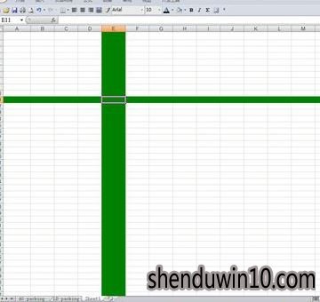
大家可以改ColorIndex,直到出现满意的颜色。以下是截图:
WPS Excel设置方法:
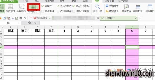
1、首先我们进入“视图”界面;
2、在视图界面,找到“阅读模式”,点击即可开启阅读模式,如图:
以上就是电脑excel点击单元格出现十字怎么如何设置的教程的详细内容了,相信大家会有用的!
office Excel设置方法:
1、打开excel,然后按下ALT+F11,会出现Microsoft Visual Basic界面;
2、在弹出的创建中键入下面代码:
Private Sub Worksheet_SelectionChange(ByVal Target As Range)
If Target.EntireColumn.Address = Target.Address Then
Cells.Interior.ColorIndex = xlNone
Exit Sub
End If
If Target.EntireRow.Address = Target.Address Then
Cells.Interior.ColorIndex = xlNone
Exit Sub
End If
Cells.Interior.ColorIndex = xlNone
Rows(Selection.Row & ":" & Selection.Row + Selection.Rows.Count - 1).Interior.ColorIndex = 10
Columns(Selection.Column).Resize(, Selection.Columns.Count).Interior.ColorIndex = 10
End Sub
大家可以改ColorIndex,直到出现满意的颜色。以下是截图:
WPS Excel设置方法:
1、首先我们进入“视图”界面;
2、在视图界面,找到“阅读模式”,点击即可开启阅读模式,如图:
以上就是电脑excel点击单元格出现十字怎么如何设置的教程的详细内容了,相信大家会有用的!
精品APP推荐
Doxillion V2.22
翼年代win8动漫主题
思维快车 V2.7 绿色版
地板换色系统 V1.0 绿色版
u老九u盘启动盘制作工具 v7.0 UEFI版
EX安全卫士 V6.0.3
清新绿色四月日历Win8主题
Ghost小助手
淘宝买家卖家帐号采集 V1.5.6.0
点聚电子印章制章软件 V6.0 绿色版
风一样的女子田雨橙W8桌面
优码计件工资软件 V9.3.8
Process Hacker(查看进程软件) V2.39.124 汉化绿色版
海蓝天空清爽Win8主题
foxy 2013 v2.0.14 中文绿色版
慵懒狗狗趴地板Win8主题
PC Lighthouse v2.0 绿色特别版
游行变速器 V6.9 绿色版
彩影ARP防火墙 V6.0.2 破解版
IE卸载工具 V2.10 绿色版
- 专题推荐
- 深度技术系统推荐
- 1深度技术Ghost Win10 x64位 多驱动纯净版2019V08(绝对激活)
- 2深度技术Ghost Win10 X32增强修正版2017V01(绝对激活)
- 3深度技术Ghost Win10 (64位) 经典装机版V2017.07月(免激活)
- 4深度技术Ghost Win10 X64 精选纯净版2021v03(激活版)
- 5萝卜家园Windows11 体验装机版64位 2021.09
- 6深度技术 Ghost Win10 x86 装机版 2016年05月
- 7深度技术Ghost Win10 x64位 特别纯净版v2018.01(绝对激活)
- 8深度技术Ghost Win10 X32位 完美装机版2017.09月(免激活)
- 9深度技术 Ghost Win10 32位 装机版 V2016.09(免激活)
- 10深度技术Ghost Win10 x64位 完美纯净版2019年05月(无需激活)
- 深度技术系统教程推荐